Support Vector Machines (SVMs)

Support Vector Machines from [LIBSVM]

class mlpy.LibSvm(svm_type='c_svc', kernel_type='linear', degree=3, gamma=0.001, coef0=0, C=1, nu=0.5, eps=0.001, p=0.1, cache_size=100, shrinking=True, probability=False, weight={})

LibSvm.

Parameters :

svm_type : string

SVM type, can be one of: ‘c_svc’, ‘nu_svc’, ‘one_class’, ‘epsilon_svr’, ‘nu_svr’

kernel_type : string

kernel type, can be one of: ‘linear’ (uT*v), ‘poly’ ((gamma*uT*v + coef0)^degree), ‘rbf’ (exp(-gamma*|u-v|^2)), ‘sigmoid’ (tanh(gamma*uT*v + coef0))

degree : int (for ‘poly’ kernel_type)

degree in kernel

gamma : float (for ‘poly’, ‘rbf’, ‘sigmoid’ kernel_type)

gamma in kernel (e.g. 1 / number of features)

coef0 : float (for ‘poly’, ‘sigmoid’ kernel_type)

coef0 in kernel

C : float (for ‘c_svc’, ‘epsilon_svr’, ‘nu_svr’)

cost of constraints violation

nu : float (for ‘nu_svc’, ‘one_class’, ‘nu_svr’)

nu parameter

eps : float

stopping criterion, usually 0.00001 in nu-SVC, 0.001 in others

p : float (for ‘epsilon_svr’)

p is the epsilon in epsilon-insensitive loss function of epsilon-SVM regression

cache_size : float [MB]

size of the kernel cache, specified in megabytes

shrinking : bool

use the shrinking heuristics

probability : bool

predict probability estimates

weight : dict

changes the penalty for some classes (if the weight for a class is not changed, it is set to 1). For example, to change penalty for classes 1 and 2 to 0.5 and 0.8 respectively set weight={1:0.5, 2:0.8}

LibSvm.learn(x, y)

Constructs the model. For classification, y is an integer indicating the class label (multi-class is supported). For regression, y is the target value which can be any real number. For one-class SVM, it’s not used so can be any number.

Parameters :

x : 2d array_like object

training data (N, P)

y : 1d array_like object

target values (N)

LibSvm.pred(t)

Does classification or regression on test vector(s) t.

Parameters :

t : 1d (one sample) or 2d array_like object

test data ([M,] P)

Returns :

p : for a classification model, the predicted class(es) for t is

returned. For a regression model, the function value(s) of t calculated using the model is returned. For an one-class model, +1 or -1 is returned.

LibSvm.pred_probability(t)

Returns C (number of classes) probability estimates. For a ‘c_svc’ and ‘nu_svc’ classification models with probability information, this method computes ‘number of classes’ probability estimates.

Parameters :

t : 1d (one sample) or 2d array_like object

test data ([M,] P)

Returns :

probability estimates : 1d (C) or 2d numpy array (M,C)

probability estimates for each observation.

LibSvm.pred_values(t)

Returns D decision values. For a classification model with C classes, this method returns D=C*(C-1)/2 decision values for each test sample. The order is label[0] vs. label[1], ..., label[0] vs. label[C-1], label[1] vs. label[2], ..., label[C-2] vs. label[C-1], where label can be obtained from the method labels().

For a one-class model, this method returns D=1 decision value for each test sample.

For a regression model, this method returns the predicted value as in pred()

Parameters :

t : 1d (one sample) or 2d array_like object

test data ([M,] P)

Returns :

decision values : 1d (D) or 2d numpy array (M,D)

decision values for each observation.

LibSvm.labels()

For a classification model, this method outputs the name of labels. For regression and one-class models, this method returns None.

LibSvm.nclasses()

Get the number of classes. = 2 in regression and in one class SVM

LibSvm.nsv()

Get the total number of support vectors.

LibSvm.label_nsv()

Return a dictionary containing the number of support vectors for each class (for classification).

static LibSvm.load_model(filename)

Loads model from file. Returns a LibSvm object with the learn() method disabled.

LibSvm.save_model(filename)

Saves model to a file.

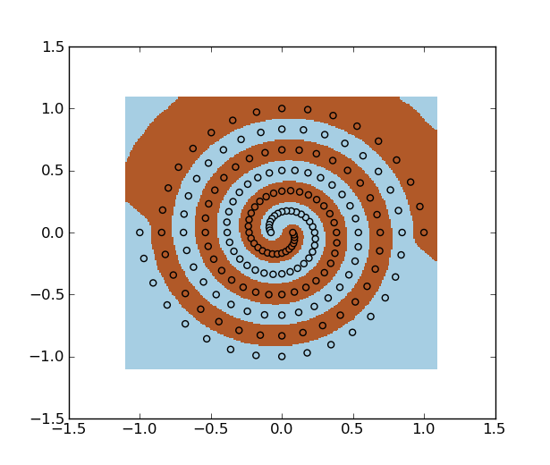
Example on spiral dataset:

>>> import numpy as np
>>> import matplotlib.pyplot as plt
>>> import mlpy
>>> f = np.loadtxt("spiral.data")
>>> x, y = f[:, :2], f[:, 2]
>>> svm = mlpy.LibSvm(svm_type='c_svc', kernel_type='rbf', gamma=100)
>>> svm.learn(x, y)
>>> xmin, xmax = x[:,0].min()-0.1, x[:,0].max()+0.1
>>> ymin, ymax = x[:,1].min()-0.1, x[:,1].max()+0.1
>>> xx, yy = np.meshgrid(np.arange(xmin, xmax, 0.01), np.arange(ymin, ymax, 0.01))
>>> xnew = np.c_[xx.ravel(), yy.ravel()]
>>> ynew = svm.pred(xnew).reshape(xx.shape)
>>> fig = plt.figure(1)
>>> plt.set_cmap(plt.cm.Paired)
>>> plt.pcolormesh(xx, yy, ynew)
>>> plt.scatter(x[:,0], x[:,1], c=y)
>>> plt.show()

[LIBSVM]

Chih-Chung Chang and Chih-Jen Lin. LIBSVM: a library for support vector machines. 2001. Software available at http://www.csie.ntu.edu.tw/~cjlin/libsvm

[Cristianini]

N Cristianini and J Shawe-Taylor. An introduction to support vector machines. Cambridge University Press.

[Vapnik95]

V Vapnik. The Nature of Statistical Learning Theory. Springer-Verlag, 1995.

Kernel Adatron

class mlpy.KernelAdatron(C=1000, maxsteps=1000, eps=0.01)

Kernel Adatron algorithm without-bias-term (binary classifier).

The algoritm handles a version of the 1-norm soft margin support vector machine. If C is very high the algoritm handles a version of the hard margin SVM.

Use positive definite kernels (such as Gaussian and Polynomial kernels)

Parameters :

C : float

upper bound on the value of alpha

maxsteps : integer (> 0)

maximum number of steps

eps : float (>=0)

the algoritm stops when abs(1 - margin) < eps

KernelAdatron.learn(K, y)

Learn.

Parameters:

K: 2d array_like object (N, N)

precomputed kernel matrix

y : 1d array_like object (N)

target values

KernelAdatron.pred(Kt)

Compute the predicted class.

Parameters :

Kt : 1d or 2d array_like object ([M], N)

test kernel matrix. Precomputed inner products (in feature space) between M testing and N training points.

Returns :

p : integer or 1d numpy array

predicted class

KernelAdatron.margin()

Return the margin.

KernelAdatron.steps()

Return the number of steps performed.

KernelAdatron.alpha()

Return alpha

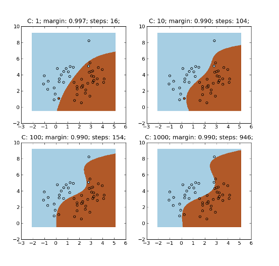
Example:

>>> import numpy as np
>>> import matplotlib.pyplot as plt
>>> import mlpy
>>> np.random.seed(0)
>>> mean1, cov1, n1 = [1, 4.5], [[1,1],[1,2]], 20  # 20 samples of class 1
>>> x1 = np.random.multivariate_normal(mean1, cov1, n1)
>>> y1 = np.ones(n1, dtype=np.int)
>>> mean2, cov2, n2 = [2.5, 2.5], [[1,1],[1,2]], 30 # 30 samples of class 2
>>> x2 = np.random.multivariate_normal(mean2, cov2, n2)
>>> y2 = 2 * np.ones(n2, dtype=np.int)
>>> x = np.concatenate((x1, x2), axis=0) # concatenate the samples
>>> y = np.concatenate((y1, y2))
>>> K = mlpy.kernel_gaussian(x, x, sigma=2) # kernel matrix
>>> xmin, xmax = x[:,0].min()-1, x[:,0].max()+1
>>> ymin, ymax = x[:,1].min()-1, x[:,1].max()+1
>>> xx, yy = np.meshgrid(np.arange(xmin, xmax, 0.02), np.arange(ymin, ymax, 0.02))
>>> xt = np.c_[xx.ravel(), yy.ravel()] # test points
>>> Kt = mlpy.kernel_gaussian(xt, x, sigma=2) # test kernel matrix
>>> fig = plt.figure(1)
>>> cmap = plt.set_cmap(plt.cm.Paired)
>>> for i, c in enumerate([1, 10, 100, 1000]):
...     ka = mlpy.KernelAdatron(C=c)
...     ax = plt.subplot(2, 2, i+1)
...     ka.learn(K, y)
...     ytest = ka.pred(Kt).reshape(xx.shape)
...     title = ax.set_title('C: %s; margin: %.3f; steps: %s;' % (c, ka.margin(), ka.steps()))
...     plot1 = plt.pcolormesh(xx, yy, ytest)
...     plot2 = plt.scatter(x[:,0], x[:,1], c=y)
>>> plt.show()

[Friess]

Friess, Cristianini, Campbell. The Kernel-Adatron Algorithm: a Fast and Simple Learning Procedure for Support Vector Machines.

[Kecman03]

Kecman, Vogt, Huang. On the Equality of Kernel AdaTron and Sequential Minimal Optimization in Classification and Regression Tasks and Alike Algorithms for Kernel Machines. ESANN‘2003 proceedings - European Symposium on Artificial Neural Networks, ISBN 2-930307-03-X, pp. 215-222.