Tutorial

If you are new in Python and NumPy see: http://docs.python.org/tutorial/ http://www.scipy.org/Tentative_NumPy_Tutorial and http://matplotlib.sourceforge.net/.

A learning problem usually considers a set of p-dimensional samples (observations) of data and tries to predict properties of unknown data.

Tutorial 1 - Iris Dataset

The well known Iris dataset represents 3 kinds of Iris flowers with 150 observations and 4 attributes: sepal length, sepal width, petal length and petal width.

A dimensionality reduction and learning tasks can be performed by the mlpy library with just a few number of commands.

Download Iris dataset

Load the modules:

>>> import numpy as np
>>> import mlpy
>>> import matplotlib.pyplot as plt # required for plotting

Load the Iris dataset:

>>> iris = np.loadtxt('iris.csv', delimiter=',')
>>> x, y = iris[:, :4], iris[:, 4].astype(np.int) # x: (observations x attributes) matrix, y: classes (1: setosa, 2: versicolor, 3: virginica)
>>> x.shape
(150, 4)
>>> y.shape
(150, )

Dimensionality reduction by Principal Component Analysis (PCA)

>>> pca = mlpy.PCA() # new PCA instance
>>> pca.learn(x) # learn from data
>>> z = pca.transform(x, k=2) # embed x into the k=2 dimensional subspace
>>> z.shape
(150, 2)

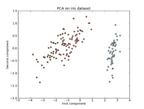
Plot the principal components:

>>> plt.set_cmap(plt.cm.Paired)
>>> fig1 = plt.figure(1)
>>> title = plt.title("PCA on iris dataset")
>>> plot = plt.scatter(z[:, 0], z[:, 1], c=y)
>>> labx = plt.xlabel("First component")
>>> laby = plt.ylabel("Second component")
>>> plt.show()

Learning by Kernel Support Vector Machines (SVMs) on principal components:

>>> linear_svm = mlpy.LibSvm(kernel_type='linear') # new linear SVM instance
>>> linear_svm.learn(z, y) # learn from principal components

For plotting purposes, we build the grid where we will compute the predictions (zgrid):

>>> xmin, xmax = z[:,0].min()-0.1, z[:,0].max()+0.1
>>> ymin, ymax = z[:,1].min()-0.1, z[:,1].max()+0.1
>>> xx, yy = np.meshgrid(np.arange(xmin, xmax, 0.01), np.arange(ymin, ymax, 0.01))
>>> zgrid = np.c_[xx.ravel(), yy.ravel()]

Now we perform the predictions on the grid. The pred() method returns the prediction for each point in zgrid:

>>> yp = linear_svm.pred(zgrid)

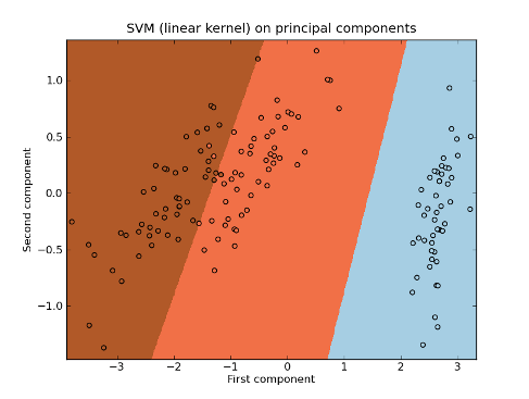
Plot the predictions:

>>> plt.set_cmap(plt.cm.Paired)
>>> fig2 = plt.figure(2)
>>> title = plt.title("SVM (linear kernel) on principal components")
>>> plot1 = plt.pcolormesh(xx, yy, yp.reshape(xx.shape))
>>> plot2 = plt.scatter(z[:, 0], z[:, 1], c=y)
>>> labx = plt.xlabel("First component")
>>> laby = plt.ylabel("Second component")
>>> limx = plt.xlim(xmin, xmax)
>>> limy = plt.ylim(ymin, ymax)
>>> plt.show()

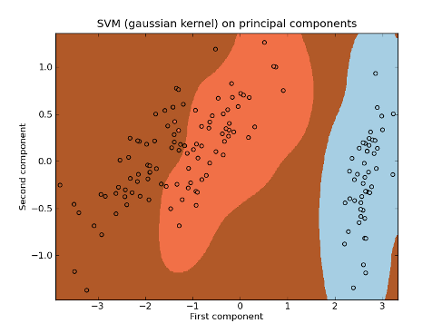
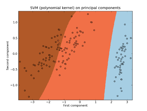
We can try to use different kernels to obtain: