Linear Methods for Regression
Ordinary Least Squares
- mlpy.ols_base(x, y, tol)
Ordinary (Linear) Least Squares.
Solves the equation X beta = y by computing a vector beta that minimize ||y - X beta||^2 where ||.|| is the L^2 norm This function uses numpy.linalg.lstsq().
X must be centered by columns.
Parameters : - x : 2d array_like object
training data (samples x features)
- y : 1d array_like object integer (two classes)
target values
- tol : float
Cut-off ratio for small singular values of x. Singular values are set to zero if they are smaller than tol times the largest singular value of x. If tol < 0, machine precision is used instead.
Returns : - beta, rank = 1d numpy array, float
beta, rank of matrix x.
- class mlpy.OLS(tol=-1)
Ordinary (Linear) Least Squares Regression (OLS).
Initialization.
Parameters : - tol : float
Cut-off ratio for small singular values of x. Singular values are set to zero if they are smaller than tol times the largest singular value of x. If tol < 0, machine precision is used instead.
- beta()
Return b1, ..., bp.
- beta0()
Return b0.
- learn(x, y)
Learning method.
Parameters : - x : 2d array_like object
training data (samples x features)
- y : 1d array_like object integer (two classes)
target values
- pred(t)
Compute the predicted response.
Parameters : - t : 1d or 2d array_like object
test data
Returns : - p : integer or 1d numpy darray
predicted response
- rank()
Rank of matrix x.
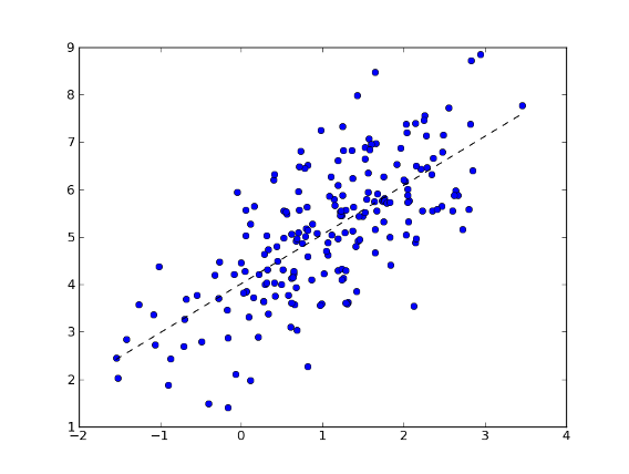
Example:
>>> import numpy as np
>>> import matplotlib.pyplot as plt
>>> import mlpy
>>> np.random.seed(0)
>>> mean, cov, n = [1, 5], [[1,1],[1,2]], 200
>>> d = np.random.multivariate_normal(mean, cov, n)
>>> x, y = d[:, 0].reshape(-1, 1), d[:, 1]
>>> x.shape
(200, 1)
>>> ols = mlpy.OLS()
>>> ols.learn(x, y)
>>> xx = np.arange(np.min(x), np.max(x), 0.01).reshape(-1, 1)
>>> yy = ols.pred(xx)
>>> fig = plt.figure(1) # plot
>>> plot = plt.plot(x, y, 'o', xx, yy, '--k')
>>> plt.show()

Ridge Regression
See [Hoerl70]. Ridge regression is also known as regularized least
squares. It avoids overfitting by controlling the size of the model vector
 , measured by its
  -norm.
- mlpy.ridge_base(x, y, lmb)
Solves the equation X beta = y by computing a vector beta that minimize ||y - X beta||^2 + ||lambda beta||^2 where ||.|| is the L^2 norm (X is a NxP matrix). When if N >= P the function solves the normal equation (primal solution), when N < P the function solves the dual solution.
X must be centered by columns.
Parameters : - x : 2d array_like object
training data (N x P)
- y : 1d array_like object (N)
target values
- lmb : float (> 0.0)
lambda, regularization parameter
Returns : - beta : 1d numpy array
beta
- class mlpy.Ridge(lmb=1.0)
Ridge Regression.
Solves the equation X beta = y by computing a vector beta that minimize ||y - X beta||^2 + ||lambda beta||^2 where ||.|| is the L^2 norm (X is a NxP matrix). When if N >= P the function solves the normal equation (primal solution), when N < P the function solves the dual solution.
Initialization.
Parameters : - lmb : float (>= 0.0)
regularization parameter
- beta()
Return b1, ..., bp.
- beta0()
Return b0.
- learn(x, y)
Compute the regression coefficients.
- Parameters:
- x : 2d array_like object
- training data (N x P)
- y : 1d array_like object (N)
- target values
- pred(t)
Compute the predicted response.
Parameters : - t : 1d or 2d array_like object ([M,] P)
test data
Returns : - p : integer or 1d numpy darray
predicted response
Example:
>>> import numpy as np
>>> import matplotlib.pyplot as plt
>>> import mlpy
>>> np.random.seed(0)
>>> mean, cov, n = [1, 5], [[1,1],[1,2]], 200
>>> d = np.random.multivariate_normal(mean, cov, n)
>>> x, y = d[:, 0].reshape(-1, 1), d[:, 1]
>>> x.shape
(200, 1)
>>> ridge = mlpy.Ridge()
>>> ridge.learn(x, y)
>>> xx = np.arange(np.min(x), np.max(x), 0.01).reshape(-1, 1)
>>> yy = ridge.pred(xx)
>>> fig = plt.figure(1) # plot
>>> plot = plt.plot(x, y, 'o', xx, yy, '--k')
>>> plt.show()

Last Angle Regression (LARS)
- mlpy.lars_base(x, y, maxsteps=None)
Least Angle Regression.
x should be centered and normalized by columns, and y should be centered.
Parameters: - x : 2d array_like object (N x P)
matrix of regressors
- y : 1d array_like object (N)
response
- maxsteps : int (> 0) or None
maximum number of steps. If maxsteps is None, the maximum number of steps is min(N-1, P), where N is the number of variables and P is the number of features.
Returns: - active, est, steps : 1d numpy array, 2d numpy array, int
active features, all LARS estimates, number of steps performed
- class mlpy.LARS(maxsteps=None)
Least Angle Regression.
Initialization.
Parameters : - maxsteps : int (> 0) or None
maximum number of steps.
- active()
Returns the active features.
- beta()
Return b_1, ..., b_p.
- beta0()
Return b_0.
- est()
Returns all LARS estimates.
- learn(x, y)
Compute the regression coefficients.
Parameters : - x : 2d array_like object (N x P)
matrix of regressors
- y : 1d array_like object (N)
response
- pred(t)
Compute the predicted response.
Parameters : - t : 1d or 2d array_like object ([M,] P)
test data
Returns : - p : float or 1d numpy array
predicted response
- steps()
Return the number of steps performed.
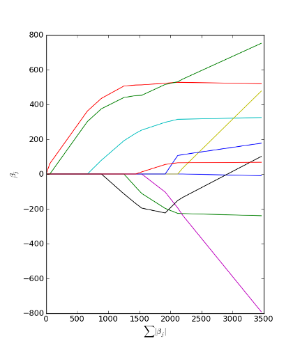
This example replicates the Figure 3 in [Efron04]. The diabetes data can be downloaded from http://www.stanford.edu/~hastie/Papers/LARS/diabetes.data
>>> import numpy as np
>>> import matplotlib.pyplot as plt
>>> import mlpy
>>> diabetes = np.loadtxt("diabetes.data", skiprows=1)
>>> x = diabetes[:, :-1]
>>> y = diabetes[:, -1]
>>> x -= np.mean(x, axis=0) # center x
>>> x /= np.sqrt(np.sum((x)**2, axis=0)) # normalize x
>>> y -= np.mean(y) # center y
>>> lars = mlpy.LARS()
>>> lars.learn(x, y)
>>> lars.steps() # number of steps performed
10
>>> lars.beta()
array([ -10.0098663 , -239.81564367,  519.84592005,  324.3846455 ,
       -792.17563855,  476.73902101,  101.04326794,  177.06323767,
        751.27369956,   67.62669218])
>>> lars.beta0()
4.7406304540474682e-14
>>> est = lars.est() # returns all LARS estimates
>>> beta_sum = np.sum(np.abs(est), axis=1)
>>> fig = plt.figure(1)
>>> plot1 = plt.plot(beta_sum, est)
>>> xl = plt.xlabel(r'$\sum{|\beta_j|}$')
>>> yl = plt.ylabel(r'$\beta_j$')
>>> plt.show()

Elastic Net
Documentation and implementation is taken from http://web.mit.edu/lrosasco/www/contents/code/ENcode.html
Computes the coefficient vector which solves the elastic-net regularization problem

Elastic Net Regularization is an algorithm for learning and variable selection. It is based on a regularized least square procedure with a penalty which is the sum of an L1 penalty (like Lasso) and an L2 penalty (like ridge regression). The first term enforces the sparsity of the solution, whereas the second term ensures democracy among groups of correlated variables. The second term has also a smoothing effect that stabilizes the obtained solution.
- mlpy.elasticnet_base(x, y, lmb, eps, supp=True, tol=0.01)
Elastic Net Regularization via Iterative Soft Thresholding.
x should be centered and normalized by columns, and y should be centered.
Computes the coefficient vector which solves the elastic-net regularization problem min {|| X beta - Y ||^2 + lambda(|beta|^2_2 + eps |beta|_1}. The solution beta is computed via iterative soft-thresholding, with damping factor 1/(1+eps*lambda), thresholding factor eps*lambda, null initialization vector and step 1 / (eig_max(XX^T)*1.1).
Parameters : - x : 2d array_like object (N x P)
matrix of regressors
- y : 1d array_like object (N)
response
- lmb : float
regularization parameter controlling overfitting. lmb can be tuned via cross validation.
- eps : float
correlation parameter preserving correlation among variables against sparsity. The solutions obtained for different values of the correlation parameter have the same prediction properties but different feature representation.
- supp : bool
if True, the algorithm stops when the support of beta reached convergence. If False, the algorithm stops when the coefficients reached convergence, that is when the beta_{l}(i) - beta_{l+1}(i) > tol * beta_{l}(i) for all i.
- tol : double
tolerance for convergence
Returns : - beta, iters : 1d numpy array, int
beta, number of iterations performed
- class mlpy.ElasticNet(lmb, eps, supp=True, tol=0.01)
Elastic Net Regularization via Iterative Soft Thresholding.
Computes the coefficient vector which solves the elastic-net regularization problem min {|| X beta - Y ||^2 + lambda(|beta|^2_2 + eps |beta|_1}. The solution beta is computed via iterative soft-thresholding, with damping factor 1/(1+eps*lambda), thresholding factor eps*lambda, null initialization vector and step 1 / (eig_max(XX^T)*1.1).
Initialization.
Parameters : - lmb : float
regularization parameter controlling overfitting. lmb can be tuned via cross validation.
- eps : float
correlation parameter preserving correlation among variables against sparsity. The solutions obtained for different values of the correlation parameter have the same prediction properties but different feature representation.
- supp : bool
if True, the algorithm stops when the support of beta reached convergence. If False, the algorithm stops when the coefficients reached convergence, that is when the beta_{l}(i) - beta_{l+1}(i) > tol * beta_{l}(i) for all i.
- tol : double
tolerance for convergence
- beta()
Return b_1, ..., b_p.
- beta0()
Return b_0.
- iters()
Return the number of iterations performed.
- learn(x, y)
Compute the regression coefficients.
Parameters : - x : 2d array_like object (N x P)
matrix of regressors
- y : 1d array_like object (N)
response
- pred(t)
Compute the predicted response.
Parameters : - t : 1d or 2d array_like object ([M,] P)
test data
Returns : - p : float or 1d numpy array
predicted response
| [DeMol08] | C De Mol, E De Vito and L Rosasco. Elastic Net Regularization in Learning Theory,CBCL paper #273/ CSAILTechnical Report #TR-2008-046, Massachusetts Institute of Technology, Cambridge, MA, July 24, 2008. arXiv:0807.3423 (to appear in the Journal of Complexity). |
| [Efron04] | Bradley Efron, Trevor Hastie, Iain Johnstone and Robert Tibshirani. Least Angle Regression. Annals of Statistics, 2004, volume 32, pages 407-499. |
| [Hoerl70] | A E Hoerl and R W Kennard. Ridge Regression: Biased Estimation for Nonorthogonal Problems. Technometrics. Vol. 12, No. 1, 1970, pp. 55–67. |