Large Linear Classification from [LIBLINEAR]
Solvers:
- L2-regularized logistic regression (primal) - l2r_lr
- L2-regularized L2-loss support vector classification (dual) - l2r_l2loss_svc_dual
- L2-regularized L2-loss support vector classification (primal) - l2r_l2loss_svc
- L2-regularized L1-loss support vector classification (dual) - l2r_l1loss_svc_dual
- multi-class support vector classification by Crammer and Singer - mcsvm_cs
- L1-regularized L2-loss support vector classification - l1r_l2loss_svc
- L1-regularized logistic regression - l1r_lr
- L2-regularized logistic regression (dual) - l2r_lr_dual
- class mlpy.LibLinear(solver_type='l2r_lr', C=1, eps=0.01, weight={})
LibLinear.
Parameters : - solver_type : string
solver, can be one of ‘l2r_lr’, ‘l2r_l2loss_svc_dual’, ‘l2r_l2loss_svc’, ‘l2r_l1loss_svc_dual’, ‘mcsvm_cs’, ‘l1r_l2loss_svc’, ‘l1r_lr’, ‘l2r_lr_dual’
- C : float
cost of constraints violation
- eps : float
stopping criterion
- weight : dict
changes the penalty for some classes (if the weight for a class is not changed, it is set to 1). For example, to change penalty for classes 1 and 2 to 0.5 and 0.8 respectively set weight={1:0.5, 2:0.8}
- LibLinear.learn(x, y)
Constructs the model.
Parameters : - x : 2d array_like object
training data (samples x features)
- y : 1d array_like object
target values
- LibLinear.pred(t)
Does classification on test vector(s) t.
Parameters : - t : 1d (one sample) or 2d array_like object
test data
Returns : - p : int or 1d numpy array
the predicted class(es) for t is returned.
- LibLinear.w()
Returns the coefficients. For ‘mcsvm_cs’ solver and for multiclass classification this method returns a 2d numpy array where w[i] contains the coefficients of label i. For binary classification an 1d numpy array is returned.
- LibLinear.bias()
Returns the bias term(s). For ‘mcsvm_cs’ solver and for multiclass classification this method returns a 1d numpy array where b[i] contains the bias of label i (.labels()[i]). For binary classification a float is returned.
- LibLinear.nfeature()
Returns the number of attributes.
- LibLinear.nclasses()
Returns the number of classes.
- LibLinear.labels()
Outputs the name of labels.
- static LibLinear.load_model(filename)
Loads model from file. Returns a LibLinear object with the learn() method disabled.
- LibLinear.save_model(filename)
Saves a model to a file.
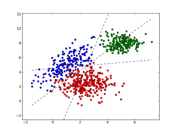
Example:
>>> import numpy as np
>>> import matplotlib.pyplot as plt
>>> import mlpy
>>> np.random.seed(0)
>>> mean1, cov1, n1 = [1, 5], [[1,1],[1,2]], 200  # 200 samples of class 0
>>> x1 = np.random.multivariate_normal(mean1, cov1, n1)
>>> y1 = np.zeros(n1, dtype=np.int)
>>> mean2, cov2, n2 = [2.5, 2.5], [[1,0],[0,1]], 300 # 300 samples of class 1
>>> x2 = np.random.multivariate_normal(mean2, cov2, n2)
>>> y2 = np.ones(n2, dtype=np.int)
>>> mean3, cov3, n3 = [5, 8], [[0.5,0],[0,0.5]], 200 # 200 samples of class 2
>>> x3 = np.random.multivariate_normal(mean3, cov3, n3)
>>> y3 = 2 * np.ones(n3, dtype=np.int)
>>> x = np.concatenate((x1, x2, x3), axis=0) # concatenate the samples
>>> y = np.concatenate((y1, y2, y3))
>>> svm = mlpy.LibLinear(solver_type='l2r_l2loss_svc_dual', C=0.01)
>>> svm.learn(x, y)
>>> w = svm.w() # w[i]: coefficients for label svm.labels()[i]
>>> w
array([[-0.73225278,  0.33309388],
       [ 0.32295557, -0.44097029],
       [ 0.23192595,  0.11536679]])
>>> b = svm.bias() # b[i]: bias for label svm.labels()[i]
>>> b
array([-0.21631629,  0.96014472, -1.53933202])
>>> xx = np.arange(np.min(x[:,0]), np.max(x[:,0]), 0.01)
>>> yy1 = (xx* (w[1][0]-w[0][0]) + b[1] - b[0]) / (w[0][1]-w[1][1])
>>> yy2 = (xx* (w[2][0]-w[0][0]) + b[2] - b[0]) / (w[0][1]-w[2][1])
>>> yy3 = (xx* (w[2][0]-w[1][0]) + b[2] - b[1]) / (w[1][1]-w[2][1])
>>> fig = plt.figure(1) # plot
>>> plot1 = plt.plot(x1[:, 0], x1[:, 1], 'ob', x2[:, 0], x2[:, 1], 'or', x3[:, 0], x3[:, 1], 'og')
>>> plot2 = plt.plot(xx, yy1, '--k')
>>> plot3 = plt.plot(xx, yy2, '--k')
>>> plot4 = plt.plot(xx, yy3, '--k')
>>> plt.show()

>>> test = [[6,7], [4, 2]] # test points
>>> print svm.pred(test)
array([2, 1])
| [LIBLINEAR] | Machine Learning Group at National Taiwan University. http://www.csie.ntu.edu.tw/~cjlin/liblinear/ |